Tuesday, June 21, 2011

Numerical variables profiling in very large data set

Profiling numerical variables is an integral part of data analytics, which generally consists of obtaining standard descriptive statistics such as quantiles, first central moments as well as missing ratio.

It is easily obtainable by using PROC MEANS (or PROC SUMMARY). But when we face very large data with many varibles, we will hit memory wall and very long processing time using default options in PROC MEANS. The most time consuming and memory intensive descriptive statistics is quantile calculation. The default method uses ordered statistics, which is the most accurate but also the most memory intensive and time consuming one.

There are two methods available to handle this scenario, both uses the one-pass method of Jain R. and Chlamtac I [1]. This method is able to obtain fairly accurate estimate of quantiles between P25 and P75, but for quantiles outside this range, the estimates will be more rough but given very large sample, maybe acceptable. Another problem is that this estimator is sensitive to the distribution of underlying data [2]. There are newer methods available that are insensitive to the distribution, such as [3].

In PROC MEANS, we can specify QMETHOD=P2 or QMETHOD=HIST to call this one pass method. Or we can use PROC STDIZE, specifying PCTLMTD=ONEPASS to invoke P2 method to calculate quantiles. Each has its pro and con.

PROC MEANS:
PRO: Multithreaded / rich set of descriptive statistics;
CON: Only pre-defined quantiles, output data set is not user friendly, in need of further manipulation;

PROC STDIZE:
PRO: quantiles of 0 to 100 are available, statistics output data is in a user friendly format;
CON: No multithreads, lack of higher central moments statistics, need to surpress data output explicitly;

Of couse, due to the way the output statistics are organized from PROC STDIZE OUTSTAT=, it can be parallelized very easily, and by examining the actual CPU time, PROC STDIZE is more efficient than PROC MEANS. Besides, higher central moments can be calculated from obtained first 2 central moments and this is done in the small output data set.

Below the difference between default method and the two new approaches is illustrated.


options fullstimer;
data test;
        length id 8;
  array x{100} ;
  do id=1 to 1e5;
      do j=1 to dim(x); x[j]=rannor(0)*1.2; end;
   output;
   drop j;
  end;
run;


proc means data=test noprint q1  qmethod=os;
        var x1-x100;
  output  out=_mean
             mean=mean1-mean100
                   std=std_x1-std_x100
                   q1=q1_x1-q1_x100
                   p95=p95_x1-p95_x100;
run;

proc means data=test noprint q1  qmethod=p2   qmarkers=211;
        var x1-x100;
  output  out=_mean
             mean=mean1-mean100
                   std=std_x1-std_x100
                   q1=q1_x1-q1_x100
                   p95=p95_x1-p95_x100;
run;

ods select none;
proc stdize data=test  
                   out=_null_  outstat=_stat  pctlmtd=onepass  
       nmarkers=211
                   pctlpts=1 5  10  25 50  75  90  95   99;
         var x1-x100;
run;
ods select all;

Take a look at the log:


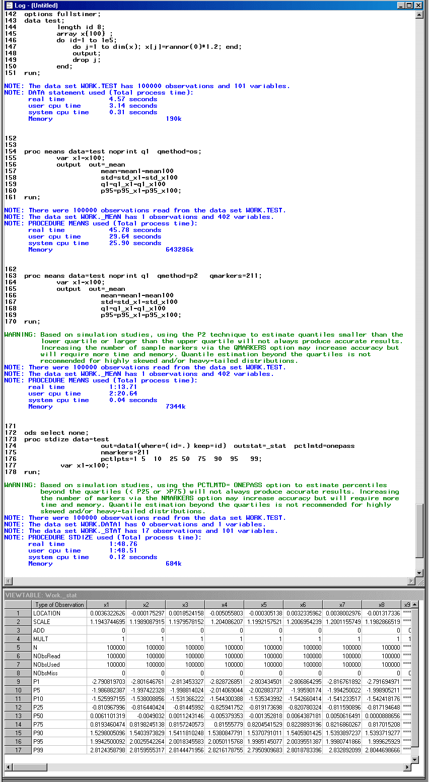
Due to smaller sample size, the most gain is on the memory side. Default approach of PROC MEANS used 643MB memory, which specifying QMETHOD=P2, the memory usage reduced to only 7.3MB. The most memory efficient is PROC STDIZE with PCTLMTD=ONEPASS, only 0.68MB memory was used.

We also examine the difference on quantile estimates using the Ordered Statistics (OS) method and P2 method in PROC MEANS. There are observable differences but not that significant:


Reference:
[1]. Jain R. and Chlamtac I. (1985), "The Algorithm for Dynamic Calculation of Quantiles and Histograms Without Storing Observations," Communications of the ACM, 28(10), 1076–1085.
[2]. SAS/STAT(R) 9.2 User's Guide, Second Edition
[3]. Alsabti, Khaled; Ranka, Sanjay; and Singh, Vineet (1997), "A One-Pass Algorithm for Accurately Estimating Quantiles for Disk-Resident Data". L.C. Smith College of Engineering and Computer Science - Former Departments, Centers, Institutes and Projects. Paper 4. http://surface.syr.edu/lcsmith_other/4

Tuesday, June 07, 2011

%HPGLIMMIX macro on large scale HMM

* Update: The SAS code and associated paper are now published at Journal of Statistical Software .
========================================================================

PROC GLIMMIX is good tool for generalized linear mixed model (GLMM), when the scale is small to medium. When facing a large scale GLMM, such as modeling all ZIPs nested in Counties nested in all 51 States in US, a 64-bit machine with extremely large memory is required and the computing may last for months! In fact, more often than not, the modeler will encounter situation where PROC GLIMMIX reports in log:

ERROR: Integer overflow on computing amount of memory required.

NOTE: The SAS System stopped processing this step because of insufficient memory.


In a strictly nested hierarchical model, however, the variance covariance matrix is very sparse, and taking advantage of this property can accelerate computing by many folds.

The %HPGLIMMIX SAS macro is made for large scale Hierarchical Mixed Models, and stands for High Performance GLIMMIX. As an example, a sample data using Gamma Regression is shown below, with all ZIPs in AK, AL, AR, AZ with 2-level hierarchies: State and ZIP within State, total 4 blocks with max 693 columns per block. The reason not all ZIPs and all states are used is simply because PROC GLIMMI blows up on the machine.

Copmaring the estimates and std errors from both runs, they are the same, but drastically different running time of 71sec using %HPGLIMMIX v.s. 35min39sec using GLIMMIX.


1715
1716  options nomprint nomlogic;
1717  %hpglimmix(data=temp2,
1718             stmts=%str(
1719                    class zip  zip_state;
1720                    model y = x ;
1721                    random int zip/subject=zip_state;
1722                      ),
1723             error=gamma,
1724             link=LOG,
1725             options=NOTEST);
NOTEST

       The HPGLIMMIX Macro

Data Set           : WORK.TEMP2
Error Distribution : GAMMA
Link Function      : LOG
Response Variable  : Y


Job Starts at : 06JUN2011:15:51:19
    HPGLIMMIX Iteration History

Iteration    Convergence criterion
    1            0.0081058432  13 sec
    2            0.0004213646  13 sec
    3            2.7137935E-7  13 sec
    4            3.1854799E-9  12 sec

Output from final Proc HPMixed run:
Job Ends at : 06JUN2011:15:52:30
1726  options nomprint nomlogic;
1727
1728  proc glimmix data=temp2;
1729       class zip  zip_state;
1730       model y = x /s  dist=gamma;
1731       random int zip /subject=zip_state;
1732  run;


NOTE: Convergence criterion (PCONV=1.11022E-8) satisfied.
NOTE: PROCEDURE GLIMMIX used (Total process time):
      real time           35:38.93
      cpu time            34:30.90


GLIMMIX output:


              Covariance Parameter Estimates

                                                  Standard
             Cov Parm     Subject      Estimate     Error

             Intercept    zip_state    0.000152    0.000125
             zip          zip_state    0.000066    3.105E-6
             Residual                  0.000405    2.281E-6

             Solutions for Fixed Effects

                                Standard
     Effect       Estimate       Error       DF    t Value    Pr > |t|

    Intercept      6.5873    0.006180        3    1065.95      <.0001
    x              0.003436    0.000218    62634      15.79      <.0001


%HPGLIMMIX output:

                _cov data from  HPGLIMMIX

               Obs    CovParm       Subject     Estimate

                1     Intercept    zip_state    0.000152
                2     zip          zip_state    0.000066
                3     Residual                  0.000405

               _soln data from HPGLIMMIX

               Obs    Effect       Estimate      StdErr

                1     Intercept      6.5873      0.006180
                2     x              0.003436    0.000218