
The data is pre-processed from raw images using NIST standardization program, but it noteworthy some extra efforts to conduct more exploratory data analysis (EDA). Because this is a pre-processed data, therefore no missing data issues and EDA will focus on descriptive statistics of input variables. The code below read in the data which is stored in folder "D:\DATA\MNIST";
%let folder=D:\Data\MNIST; libname digits "&folder"; data digits.MNISTtrain; infile "&folder.\train.csv" lrecl=32567 dlm=',' firstobs=2; input label x1-x784; run; data digits.MNISTtest; infile "&folder.\test.csv" lrecl=32567 dlm=',' firstobs=2; input x1-x784; run; Figure 1 below shows the distribution of variances of input variables in the Training set. Apparently there are many input variables of little information and they should be removed before further data processing and actual modeling. Next we examine Coefficient of Variation (CoV) of input variables. CoV gives a more consistent way to compare across variables. The result is demonstrated in figure 2. Note that variables with 0 variance will have their CoV be set to 0.
ods select none; proc means data=digits.MNISTtrain ; var x1-x784; output out=stat(where=(_STAT_ in ('STD', 'MEAN'))); run; ods select all; proc transpose data=stat out=stat_t; var _STAT_ x:; run; data stat_t; set stat_t; ID=_n_-1; if col2=0 then CoV=0; else CoV=col1/col2; run; proc sgplot data=stat_t; scatter y=col2 x=ID; label ID="X #" col2="StdErr"; run; proc sgplot data=stat_t; scatter y=CoV x=ID; label ID="X #"; run; 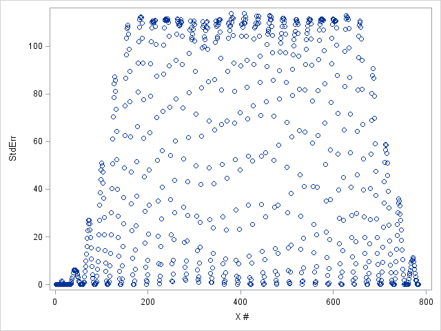 |
| Figure 1. StdErr by input features |
 |
| Figure 2. Coefficient of Variation by input features |
In this demonstration, we select features that have a variance larger than 10% of quantiles. Even so, we still end up with more than 700 features. Note that in SAS, the computing time of kNN classification increases in superlinear and kNN itself suffers curse of dimensionality, therefore it is desirable to conduct dimension reduction first before applying kNN classifiers. While there are so many different techniques to choose from, we decided to go with SVD, which is both widely used and simple to implement in SAS, see here for sample code and examples. The code below applies SVD to the data that combining both training and testing. This is important because SVD is sensitive to input data and include both data sets in the computing won't violate any best practice rules in predictive model because no information from dependent variable is used. The left eigenvectors are also standardized to have 0 mean and unit standard deviation.
data all;
set digits.MNISTtrain(in=_1)
digits.MNISTtest(in=_2);
if _1 then group='T';
else group='S';
run;
proc princomp data=all out=allpca(drop=x:) outstat=stat noint cov noprint;
var x1-x784;
run;
proc standard data=allpca out=allpcastd mean=0 std=1;
var Prin:;
run;
data allpcastd;
set allpcastd;
array _p{*} p1-p10 (10*0.1);
cv=rantbl(97897, of _p[*]);
drop p1-p10;
run;
After the data is compressed, we split them into 10 folds of subsets, flag each of them and search for best tuning parameter. In building a simple kNN classifier, there are two tuning parameters to decide, 1.what features to use and 2. the number of neighbors to use. In this exercise, we simplify the first problem into searching for the number of features, always starting from feature #1. We then calculate the error rate for each combination. Before we start a brutal force search, we have to understand that search through the whole space of combination of 700 features and 1 to 25 neighbors is not practical, it just takes too much time, may run for over 2 days on a regular PC. But we can narrow down to a range of number of features by testing number of features at every 10th interval, say test 1 feature, 11 features, 21 features,..., 201 features. In classification, kNN is more sensitive to features used instead of number of neighbors. The code below executes such experiment and will take about 18 hours to finish on my PC equipped with i5-3570 CPU, clocked at 3.8Ghz. In actual execution, I used my proprietary %foreach MACRO that distribute the job to 3 cores of the CPU, and shaved the total running time to only 6 hours.
/*@@@@@@@@@@ USE 10-FOLD CV @@@@@@@@@@*/
%macro loopy;
%do k=2 %to 8;
%do i=1 %to 10;
%let t0=%sysfunc(time());
options nosource nonotes;
proc discrim data=allpcastd(where=(group='T' & cv^=&i))
method=npar k=&k noprint
testdata=allpcastd(where=(group='T' & cv=&i))
testout=out(drop=Prin:)
;
class label;
var Prin1-Prin30;
run;
proc freq data=out noprint;
table label*_INTO_/out=table;
run;
proc sql;
create table _tmp as
select &i as cv, &k as K, 31 as dim, sum(PERCENT) as correct
from table
where label=_INTO_
;
quit;
%let t1=%sysfunc(time());
data _null_;
dt=round(&t1-&t0, 0.1);
call symput('dt', dt);
run;
%put k=&k i=&i time=&dt;
%if %eval(&k+&i)=3 %then %do;
data result; set _tmp; run;
%end;
%else %do;
data result; set result _tmp; run;
%end;
%end;
%end;
options source notes;
%mend;
options nosource nonotes;
%loopy;
options source notes;
proc means data=result noprint;
by k;
var correct;
output out=result_summary mean(correct)=mean std(correct)=std;
run;
 |
| Figure 3. Correct% vs. Number of Features by Number of Neighbors |
Now we see that the best possible number of features may exist somewhere between 21 to 41 while the number of neighbors has a much smaller influence except for using only 2 NN. Now we are in a good situation to conduct more greedy search over the feature space. We are going to search through all combinations of number of features from 21 to 41 at single interval and neighbors 3 to 7, which results in a total number of 120 iterations each runs over the 10 folds, and the code ran about 3 hours on my PC. The code below executes this exercise and the result is summarized in table 1. We can see that using up to 31 features and 3 nearest neighbors will be the best choice for the data at hand.
%macro loopy;
%do k=2 %to 7;
%do d=21 %to 41;
%do i=1 %to 5;
%let t0=%sysfunc(time());
options nosource nonotes;
proc discrim data=allpcastd(where=(group='T' & cv^=&i ))
method=npar k=&k noprint
testdata=allpcastd(where=(group='T'))
testout=out(drop=Prin:)
;
class label;
var Prin1-Prin&d;
run;
proc freq data=out noprint;
table label*_INTO_/out=table;
run;
proc sql;
create table _tmp as
select &i as cv, &k as K, &d as dim, sum(PERCENT) as correct
from table
where label=_INTO_
;
quit;
%let t1=%sysfunc(time());
data _null_;
dt=round(&t1-&t0, 0.1);
call symput('dt', dt);
run;
%put k=&k d=&d i=&i time=&dt;
%if %eval(&k=2) & %eval(&d=21) %then %do;
data result; set _tmp; run;
%end;
%else %do;
data result; set result _tmp; run;
%end;
%end;
%end;
%end;
options source notes;
%mend;
options nosource nonotes;
%loopy;
options source notes;
proc means data=result noprint nway;
class k dim;
var correct;
output out=result_summary2 mean(correct)=mean std(correct)=std;
run;
proc means data=result_summary2 nway noprint;
class k;
var mean;
output out=result_max idgroup(max(mean) out[1](mean std dim)=mean std dim);
run;
proc sgplot data=result ;
where i=.;
dot dim /response=correct stat=mean limitstat=stddev numstd=1 group=k;
label dim="# of Features";
run;
 |
| Figure 4. Correct% and Confidence Interval by # of features and # of neighbors. |
 |
| Table 1. Tuning Parameters Selection |
Now, re-score the data using chosen tuning parameters: up to 33 features and 3-NN, we end up an accuracy of 96.80% on the leader-board, which certainly is not the best result you can get from kNN method, but easily beat both the 1NN and ramdomForest benchmark results.
With a little bit more tweak, the accuracy from a kNN with similar parameters can be boosted to 97.7%.
No comments:
Post a Comment