Large Scale Linear Mixed Model

Update at the end:
****************************;
Bob at r4stats.com claimed that a linear mixed model with over 5 million observations and 2 million levels of random effects was fit using lme4 package in R:

I am always interested in large scale mixed model like this and would appreciate anyone who can point me to the example Bob quoted (update: Bob responded in comment, please check it out). I left a reply to Bob on his blog but no response yet. I also tried to Google this example but all examples returned are on a scale with hundreds up to 5 thousand of levels of random effects, which is very common and reasonable. While I don't have the data used in the quoted example, I decided to see how long it takes for a mixed model with similar scale to be fitted in SAS's PROC HPMIXED. Therefore I borrowed Tianlin Wang's simulated data example in his paper: All the Cows in Canada: Massive Mixed Modeling with the HPMIXED procedure in SAS 9.2. But I modified the code a little bit so that there will be 400K cows to be included in the random effect and I used SUBJECT= option to accelerate the computing with by-subject processing.


%let NFarm = 1000;
%let NAnimal = %eval(&NFarm*400);
%let Va = 4.0;
%let Ve = 8.0;
data Sim;
    keep Species Farm Animal Yield;
    array BV{&NAnimal};
    array AnimalSpecies{&NAnimal};
    array AnimalFarm{&NAnimal};
    do i = 1 to &NAnimal;
       BV {i} = sqrt(&Va)*rannor(12345);
       AnimalSpecies{i} = 1 + int( 5 *ranuni(12345));
       AnimalFarm {i} = 1 + int(&NFarm*ranuni(12345));
    end;
    do i = 1 to 40*&NAnimal;
       Animal = 1 + int(&NAnimal*ranuni(12345));
       Species = AnimalSpecies{Animal};
       Farm = AnimalFarm {Animal};
       Yield = 1 + Species
                 + Farm
                 + BV{Animal}
                 + sqrt(&Ve)*rannor(12345);
       output;
    end;
run;

proc sort data=sim; by animal species farm; run;
options fullstimer;
ods listing close;
ods select none;
proc hpmixed data=Sim;
     class Species Farm Animal;
     model Yield = Species Farm*Species /ddfm=residual;
     random animal /cl ;
     ods output SolutionR=EBV;
run;
ods listing;


For this particular model, it took more than 8 hours to be fitted on a desktop with i5-3570K CPU running at 3.8Ghz. I certainly dare not to test against a case with 2 million levels of random effects and would assume it will be a LONG LONG TIME. Note that with the original 10K levels of random effects, it took only 20 seconds to be fitted on the same machine, and I do know the time consumption is more than super-linear in the number of random effects' levels with all the computing optimization in HPMIXED.

lme4 package supports Sparse matrix techniques only on the random effect design matrix, but HPMIXED procedure supports Sparse matrix techniques to the full Mixed Model Equation, and in many applications, will perform much better:

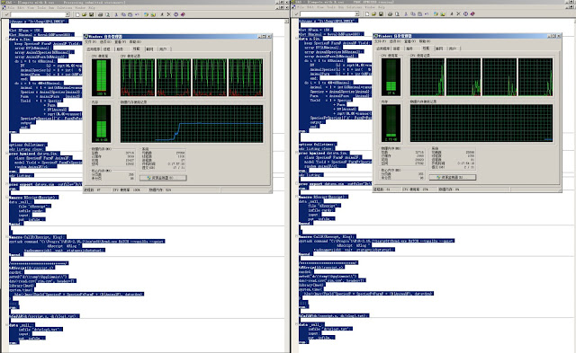
Take the above example, but using only 150 Farms and assuming 100 Animals within a Farm, we fit the same mixed model using lme4 package and the HPMIXED procedure. The lmer function is called within SAS using the %RScript and %CallR macros (see here).

Left panel shows the status of the machine running lmer function on the mixed model and the right panel shows the status when the machine ran HPMIXED. Because lme4 does not support sparse matrix techniques for fixed effect design matrix, it takes significant penalty on memory usage (12+GB vs 25MB) and computing time (244sec real time vs. 17sec real time). In a later test using only random effects, HPMIXED used 5.7 seconds while lmer used 11.3 second.

Left: Running R; Right: Running SAS