In order to illustrate this idea, Jim introduced three types of prior probability:
1. Prior probability over a discrete grid of choice, given a weight which serves as hyper-parameter;
2. Prior probability by a chosen probability. In most cases, the chosen probability is a so called conjugate prior becuase the posterior is the same family as the prior. In the book, a beta probability is chosen and it is conjugate in the sense that the posterior is also a beta distribution, only with different parameter;
3. A dense grid of prior probability choices which is called histogram prior;
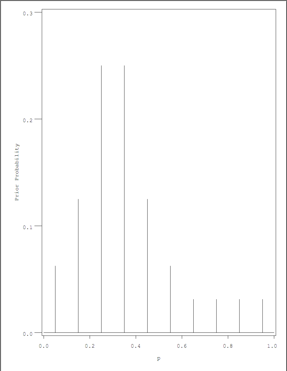
Using a discrete grid of prior choices, we first generate a list of prior probabilities, in data set PRIOR, that we believe the true proportion of heavy sleepers should be, and assign a weight, i.e. the magnitude of credibility, for each choice in a data set P, which serves as hyper-parameter. We then consolidate the two data sets into one and plot the prior against its corresponding weight.
/* Chapter 2 of Bayesian Computation with SAS */
/* In this chapter, Jim talked about applying
   Bayesian Rule to learn posterior probability
   using an example where the proportion of
   students sleeping over 8 hours a day is studies.
   Bayes Rule:
     Posterior(p|data) \prop Prior(p)* likelihood(data|p)
*/
options fullstimer formchar='|----|+|---+=|-/\<>*'  error=3;
/***************************************************/
data prior;
     input prior @@;
cards;
2 4 8 8 4 2 1 1 1 1
;
run;

data p;
     do p=0.05 to 0.95 by 0.1;
     output;
  end;
run;

data p;
     retain sum_prior 0;
     do until (eof1);
        set prior end=eof1;
        sum_prior+prior;
     end;
     do until (eof2);
        merge p  prior  end=eof2;
        prior=prior/sum_prior;
        drop sum_prior;
        output;
     end;
run;

goptions reset=all;
symbol  interpol=Needle  value=none  line=1 color=black;
axis1   label=(angle=90  'Prior Probability') order=(0 to 0.3 by 0.1) minor=none;
axis2   label=('p')   order=(0 to 1 by 0.2)  minor=none;
proc gplot data=p;
      plot prior*p /vaxis=axis1  haxis=axis2;
run;quit;
Next, we calculate the posterior probability given prior and likelihood conditional on prior. In the code below, we observe 11 heavy sleepers out of a total sample of 27. The first DATA STEP calculates the likelihood conditional on each prior choice, the posterior is output in the data set P2, where the normalization factor is the sum of conditional likelihood, scaled by max likelihood for numerical stability. You can observe the shape of posterior against hyper-parameter using GPLOT. The INTERPOL=NEEDLE option in SYMBOL statement minic the histogram style line of PLOT function in R.
%let n0=16;
%let n1=11;

data p;
     set p  end=eof1  nobs=ntotal;
     if p>0 & p<1 then do;
        log_like=log(p)*&n1 + log(1-p)*&n0;
     end;
     else
        log_like=-999*(p=0)*(&n1>0) + (p=1)*(&n0>0);
     log_posterior=log(prior) + log_like;
     if log_posterior>max_like then max_like=log_posterior;
run;

proc means data=p  noprint;
     var log_posterior;
     output out=_max  max(log_posterior)=max;
run;

data p2;
     set _max;
     sum_post=0;
     do until (eof);
        set p  end=eof;
        sum_post+exp(log_posterior-max);
     end;
     do until (eof2);
        set p end=eof2;
        posterior=exp(log_posterior-max)/sum_post;
        output;
        keep p prior  posterior;
     end;
run;

goptions reset=all;
symbol value=NONE interpol=Needle;
axis1  label=(angle=90  'Posterior Probability');
axis2  label=('p');
proc gplot data=p2;
      plot  posterior*p /vaxis=axis1  haxis=axis2;
run;quit;

After tried discrete grid of prior, beta conjugate prior is introduced. Jim mentioned that by matching the believed 50% and 90% percentiles, the parameter of prior beta distribution can be obtained by try-and-error approach. We note that the believed percentiles data indicates that the beta distribution skewed to 0, so that parameter alpha is less than parameter beta and we can use a binary search to nail down the values, which I came down to approximately 3.4 and 7.5. But I will use the {3.4, 7.4} vector as in the book. Since beta distribution is a conjugate prior for proportion, the computation is very easy. The curves for prior, likelihood and posterior are visualized.
/* beta prior */

%let a=3.4;
%let b=7.4;
%let s=11;
%let f=16;

data p;
      do i=1 to 500;
      p=i/500;
   prior=pdf('beta', p, &a, &b);
   like=pdf('beta', p, &s, &f);
   post=pdf('beta', p, &a+&s, &b+&f);
   drop i;
   output;
   end;
run;

goptions reset=all;
symbol1 interpol=j  color=red  width=1  value=none;
symbol2 interpol=j  color=blue width=2  value=none;
symbol3 interpol=j  color=gree width=3  value=none;
axis1   label=(angle=90  'Density')  order=(0 to 5 by 1) minor=none;
axis2   label=('p')      order=(0 to 1 by 0.2)  minor=none;;
legend label=none   position=(top right inside)  mode=share;
proc gplot data=p;
      plot post*p   prior*p  like*p  /overlay
                                      vaxis=axis1
                                      haxis=axis2
                                      legend=legend;
run;quit;

Since we obtain closed form for posterior distribution, we can conduct inference based on exact calculation; alternatively, we can use simulated random sample.
/* generate 1000 random obs from posterior distribution */
data rs;
      call streaminit(123456);
      do i=1 to 1000;
         x=rand('beta', &a+&s, &b+&f);
   output;
   end;
run;

proc univariate data=rs  noprint;
     var x;
     histogram /midpoints=0 to 0.8 by 0.05
                cbarline=blue  cfill=white
                outhistogram=hist;
     title "Histogram of ps";
run;
title;

axis1 label=(angle=90 "Frequency");
proc gbarline data=hist;
      bar _midpt_/discrete  sumvar=_count_  space=0  axis=axis1 ;
   title "Histogram of ps";
run;
title;

/* hist prior */
data midpt;
     do pt=0.05 to 0.95 by 0.1;
        output;
     end;
run;

In the book, Jim also mentioned using so called Histogram prior. The Histogram prior is a densed-version of discrete prior, with the distance between discrete choices filled in with dense choices of the same value, separated only by a small distance. It provides a more refined description of prior believe than the discrete prior. We plot the prior and posterior as well as random sample from posterior to give a visual impression. Note that we use PROC STDIZE method=SUM to normalize prior variable.
data prior;
input prior @@;
datalines;
2 4 8 8 4 2 1 1 1 1
;
run;
proc stdize data=prior method=sum out=prior; var prior; run;
data _null_;
set midpt nobs=ntotal1;
call symput('nmid', ntotal1);
set prior nobs=ntotal2;
call symput('nprior', ntotal2);
stop;
run;
data histprior;
array _midpt{&nmid} _temporary_;
array _prior{&nprior} _temporary_;
if _n_=1 then do;
k=1;
do until (eof1);
set midpt end=eof1;
_midpt[k]=pt; if k=2 then lo=_midpt[k]-_midpt[k-1];
k+1;
end;
do k=1 to ∤
_midpt[k]=round(_midpt[k]-lo/2, 0.00001);
put _midpt[k]=;
end;
k=1;
do until (eof2);
set prior end=eof2;
_prior[k]=prior;
put k= _prior[k]=;
if k<&nprior then k=k+1;
end;
drop k lo;
end;
do p=1/500 to 1 by 1/500;
sk=0;
do k=1 to ∤
if p>=_midpt[k] then sk=min(&nmid, sk+1);
end;
histprior=_prior[sk];
output;
end;
stop;
run;
goptions reset=all;
symbol interpol=hiloj;
axis1 label=(angle=90 "Prior Density") order=(0 to 0.3 by 0.05);
axis2 label=("p") order=(0 to 1 by 0.2);
proc gplot data=histprior;
plot histprior*p /vaxis=axis1 haxis=axis2;
run;quit;
data histposterior;
set histprior;
like=pdf('BETA',p, &s+1, &f+1);
post=like*histprior;
run;
%put &s;
goptions reset=all;
symbol interpol=hiloj;
axis1 label=(angle=90 "Posterior Density") order=(0 to 1 by 0.2);
proc gplot data=histposterior;
plot post*p/vaxis=axis1;
run;quit;
proc means data=histposterior sum;
var post;
run;
proc stdize data=histposterior method=sum out=data1;
var post;
run;
proc means data=data1 sum;
var post;
run;


In R, the SAMPLE function is able to do a URS sampling with given probability. SAS's PROC SURVEYSELECT seems can't do this with method=URS. But URS sampling with given probability is very easy to code in SAS DATA STEP with the help of FORMAT.
data fmt;
     merge histposterior(rename=(post=start))
     histposterior(firstobs=2   in=_2    rename=(post=end));
     if _2;
run;

data fmt;
     set data1   end=eof;
     retain start;
     retain fmtname 'ursp'  type 'n';
     if _n_=1 then start=post;
     else do;
        end=start+post;  label=p;
        keep  fmtname  start  end  label;
        output;
        start=end;
     end;
     if eof then do;
        hlo='O';
        label=.;
        output;
     end;
run;

proc sort data=fmt  nodupkey  out=fmt;
     by start end;
run;

proc format cntlin=fmt; run;

data  samp;
      do i=1 to 1000;
         p=input(put(ranuni(78686), ursp.), best.);
         output;
      end;
run;

proc univariate data=samp noprint;
     title "Histogram of ps";
     histogram  p/midpoints=0.15 to 0.65 by 0.05
                  outhist=samp_hist
                  vaxislabel="Frequency"  vscale=count;
run;
title;

Once we obtain posterior distribution of a variable, we can easily predict the value of some statistics given new samples. In the book, depending on the choice of weighting density, two types of predictions are discussed: 1. prior prediction; 2. posterior prediction. The calculation is straight-forward given formula.
/* prediction */
data prior;
     input prior @@;
cards;
2 4 8 8 4 2 1 1 1 1
;
run;

data p;
     do p=0.05 to 0.95 by 0.1;
     output;
  end;
run;

data p;
      retain sum_prior 0;
   do until (eof1);
      set prior end=eof1;
   sum_prior+prior;
   end;
   do until (eof2);
      merge p  prior  end=eof2;
   prior=prior/sum_prior;
   drop sum_prior;
   output;
   end;
run;

/* prediction using discrete prior */
%let m=20;
data pred;
        do ys=0 to &m;
      pred=0;
            do i=1 to 10;
                set p   point=i;
    pred = pred + prior * pdf('BINOMIAL', ys, p, &m);
    put p=  prior=  pred=  ;
   end;
   output;
  end;
  stop;
run;

/* prediction using beta(a, b) prior */
%let m=20;
%let a=3.4;
%let b=7.4;
data pred;
     do ys=0 to &m;
       pred=comb(&m, ys) *exp(logbeta(&a + ys, &b+&m -ys) - logbeta(&a, &b));
       output;
     end;
run;

/* prediction by simulation */
%let n=1000;
data pred;
        do i=1 to &n;
      p=rand('BETA', &a, &b);
   ys=rand('BINOMIAL', p, &m);
   drop i;
   output;
    end;
run;

proc freq data=pred  noprint;
        table ys /out=y_freq;
run;
/*
proc gbarline data=y_freq;
        bar y /discrete sumvar=percent;
run;quit;
*/
data y_freq;
        set y_freq;
  percent=percent/100;
  label ys='y';
run;

goptions reset=all  border;
axis1  label=(angle=90  "Predictive Probability")  order=(0 to 0.14 by 0.02);
axis2  label=("y")   order=(0 to 16) offset=(15 points, 15 points) minor=none;
symbol  interpol=needle;
proc gplot data=y_freq;
        plot  percent * ys/vaxis=axis1  haxis=axis2  ;
run;quit;

/* summarize discrete outcome with given coverage probability */
/* input dsn is y_freq from PROC FREQ. The following can be used as gauge.
data y_freq;
        input y percent;
datalines;
0  0.013
1  0.032
2  0.065
3  0.103
4  0.102
5  0.115
6  0.114
7  0.115
8  0.095
9  0.083
10 0.058
11 0.036
12 0.029
13 0.014
14 0.015
15 0.006
16 0.005
;
run;
*/
%let covprob=0.9;
proc sort data=y_freq  out=y_freq2;
        by  percent;
run;

data y_freq2;
        set y_freq2;
  retain cumprob  0;
  cumprob+percent;
  if cumprob<(1-&covprob) then select=0;
  else select=1;
run;

proc means data=y_freq2  sum;
       where select=1;
    var percent;
run;

In Summary:
0. There different choices for specifying Prior believe that can be incorporated into Bayesian computation:
a.) A discrete grid of possible values, each value with some probability
b.) An appropriate distribution, where the parameters is determined from existing information
c.) A dense grid of possible values that span the whole range
1. We demonstrated calculation under these three scenarios and their impact on posterior distribution of statistics of interests;
2. We can conduct Sampling With Replacement with given sampling probability by using FORMAT and uniform random variable generator
3. We demonstrated that prediction in a Bayesian framework is straighforward, but depending on whether we use prior distribution or posterior distribution

2 comments:
When the next chapter will be available?
Too busy recently. Writting of Chapter 3 is postponed to April.
Post a Comment